                                        CheckInWaitTime  ScanWaitTime
CTMachineScenario ReceptionistScenario
1                 1                            0.059406      0.536305
                  2                            0.000000      0.548324
2                 1                            0.059396      0.154899
2 0.000000 0.1702259 Using Traces and Scenarios
In this lab we will modify the simulation developed in the previous lab to run off of a pre-generated data trace that contains information about each patient. We will also explore how Jaamsim’s built-in scenario indices can be used to run experiments where the values of the simulation’s inputs are changed and use an EventLogger to log all events that an entity participates in. Finally we will package the simulation (Jaamsim and the custom Java code) as a .jar file, so that the simulation can be run easily from the command line on all major operating systems.
We are not considering any changes to the system, so the conceptual model is the same as for the previous lab. To have your lab signed off you need to show that you have added the data from the file to the model, exported the model as a .far file, and can run the .jar file from the command line.
9.1 Jaamsim Model
To run the simulation from a data trace we need to make some changes to the Jaamsim model. Once again create a new folder called RC3 and copy your .cfg file (and the .png files so that the graphics work) from the previous lab folder into this folder and rename it to radiology_lab_trace.cfg. First, download the RC_50_week_data.txt file from Canvas under the Lab 7: Using Traces and Scenarios Assignment. This file contains 50 weeks of data of patients at the radiology clinic including: the time the patient arrived, the priority of the patient, the time the patient took to check in, and the time the patient took to have their scan.
Before we load the data in we will first change the starting date of the simulation, which defaults to 1970, to instead be 2024, so that the data read from the file is interpreted correctly. To do this go to the Simulation object and under the Options tab enter 2024-01-01 for the StartDate.
To use the data in Jaamsim we use a FileToMatrix object found in the Basic Objects palette. Create a FileToMatrixObject, rename it PatientData, and select the RC_50_week_data.txt file as the DataFile.
We can now access the data in the file by using the Value output of the PatientData object. The first place we will use this data is in the PatientArrival object, so that patients arrive according to the data in the file, rather than the distribution used previously. We first create two CustomOutputs (under the options tab) on the PatientArrival object to make accessing the data easier. CustomOutputs are similar to attributes but they can be expressions (formulas) and are re-calculated at each time step in the simulation. The two outputs we create will correspond to the data for the patient that has just arrived (thisPatientData) and the patient that is going to arrive next (nextPatientData). We need both of these so that we can calculate the appropriate interarrival time between the patients.
Once we have created these outputs we use them in the InterArrivalTime, and AssignmentList of the PatientArrival.
| Object | Keyword | Value |
|---|---|---|
| PatientArrival | CustomOutputList | { thisPatientData ‘[PatientData].Value(this.NumberAdded + 1)’ } |
| { nextPatientData ‘[PatientData].Value(this.NumberAdded + 2)’ } | ||
| FirstArrivalTime | [PatientData].Value(2)(2) | |
| InterArrivalTime | ‘this.nextPatientData(2) - this.thisPatientData(2)’ | |
| AssignmentList | { ‘this.obj.priority= this.thisPatientData(3)’ } | |
| { ‘this.obj.checkInTime= this.thisPatientData(4)’ } | ||
| { ‘this.obj.scanTime= this.thisPatientData(5)’ } |
Note that in the AssignmentList we are assigning values from the data file to attributes on the patient entity for priority, check in time, and scan time. We will use these attributes later to determine how long those activities take (the priority attribute is already used in the PriorityBranch).
To avoid getting an error these attributes need to be added to the PatientEntity object. So update the AttributeDefinitionList of the PatientEntity to include checkInTime and scanTime as well as the current priority, all with a default of 0.
We now need to use the checkInTime and scanTime attributes to determine how long the check ins and scans take. Set the Duration of the CheckIn activity to this.CurrentParticipants(1).checkInTime * 1[min]. this.CurrentParticipants refers to the group of entities that have just started the activity (for check in this is a patient and a receptionist), and we use the index 1 as the patient comes first, then we access the checkInTime attribute. We then need to multiply this by 1[min] to convert the number into a time, and use minutes as the attribute is in minutes.
Similarly for the Scan activity set the Duration to this.CurrentParticipants(1).scanTime * 1[h], note that here we use 1[h] as the attribute is in hours.
Now, suppose we are interested in the time that patients spend waiting for check in and for the scan. We can’t use the current PatientLogger as it only records the total time that patients are in the system for. We could add attributes for each time that we are interested in, and assign the value when the entity gets to the relevant stage, and then use the PatientLogger to log these attributes. We can instead use an EventLogger from the HCCM palette. The EventLogger records the time that an entity starts each of the activities that it participates in. So, create an EventLogger and call it PatientEventLogger.
Then, to get the events recorded go to the PatientLeave object and under the HCCM tab enter PatientEventLogger for the EventLogger keyword. Now any entities that are sent to the patient leave will have the start times of any activities that they participated in recorded.
We will now configure the Simulation object to run one long replication for several scenarios. Under the Key Inputs tab enter 50w for the RunDuration, this will make the simulation run for 50 weeks. We have to run one 50 week replication rather than 50 one week replications as Jaamsim cannot read in a new file when each replication starts.
We want to try out four scenarios with either three or four CT machines, and either one or two receptionists. As there are two factors we are changing we use a ScenarioIndex with two numbers, the first indexes the scenarios relating to the number of CT Machines, and the second those related to the number of receptionists.
Since there are two options for the first index and two for the second we enter 2 2 for the ScenarioIndexDefinitionList under the MultipleRuns tab of the Simulation object. We will start from scenario 1 and end at scenario 2 in both the indices so StartingScenarioNumber is 1-1 and EndingScenarioNumber is 2-2. We are going to run just one long replication for each scenario so set the NumberOfReplications to 1.
Now Jaamsim will run 4 scenarios, but there won’t be any difference in the model in each scenario. We need to make it so that the number of CT Machines and Receptionists actually changes in each of the scenarios. For the CT Machines we set the MaxNumber and InitialNumber on the CTMachineArrival to [Simulation].ScenarioIndex(1) + 2, which gets the value of the first scenario index and adds 2 to it. For the Receptionists we can set the MaxNumber and InitialNumber on the ReceptionistArrival to [Simulation].ScenarioIndex(2), in this case we don’t need to add one as the scenario index is the same as the number of receptionists we want to use.
Now when you run the model, the number of CT Machines and Receptionists will change in each scenario.
Download and run the RC3_Analysis.R file, from Canvas under the Lab 7: Using Traces and Scenarios Assignment. You will have to update the directory that it reads the data from and the name of the data file used. The script splits each replication into 50 batches, each one week long, and calculates the mean across the batches and the four scenarios of the 90th percentile waiting time for both check in and scan within each of batch. No warm-up period is used, so this assumes that being empty and idle is a typical state of the system. Splitting into batches by week assumes that each week is not correlated to the preceding and following weeks. You should get the following output:
9.2 Creating an Executable JAR File
We can package the custom Java code in the extended control unit class alongside the base Jaamsim and HCCM code into a jar file that can be run without having to set up Java/VSCode. To do this click on the right arrow that appears when you hover over the Java Projects tab, with the tooltip ‘Export Jar’. Then in the menu that appears, select GUIFrame as the main class, then click OK with all of the options selected.
This should create a file called sim.jar inside the sim folder, alongside the hccm and sim_custom folders. Copy the sim.jar file to your folder for this lab (if you are following the structure here it is called RC3 and is in the labs folder), and rename it to RC3.jar. It doesn’t really matter where you put it, but it is much easier if the .jar file is in the same directory as the .cfg file for this lab (radiology_lab_trace.cfg).
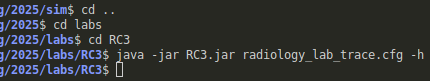
Then open a terminal in VSCode. There might be one already open, otherwise you can open one by going to Terminal in the top left, and selecting New Terminal. By default this will open a terminal in the sim folder. You will need to navigate to the folder with the .jar and .cfg files in it using the cd (change directory) command. If you are following the folder structure described then should go up one level (cd ..), then into labs (cd labs), then into RC3 (cd RC3).
Once you have a terminal open in the correct folder you can run the following command java -jar RC3.jar radiology_lab_trace.cfg -h.
This command gets java to run the RC3.jar file which then opens and runs the radiology_lab_trace.cfg model in headerless mode (denoted by the -h). Headerless mode means that the visualisation of the simulation is not shown, and allows the model to run more quickly. If it runs correctly nothing will be printed, as seen in Figure 9.1.
Once you can run the model from the command line using the .jar file (you can confirm that the model is actually running by checking the date/time modified of the output files), you can get your lab signed off.